Markov chain: What is a Markov chain?
Markov chain is a very important piece of probability and statistics. One application we could name is Markov Decision Process (MDP) used for decision making. Another one is Markov chain Monte Carlo (MCMC), a popular sampling method in statistics. You may also know Google PageRank algorithm, which is part of the ground of Google indexing technology. The algorithm is implemented on top of this concept.
This is a part of a series about Markov chain… In this post, we will look into some of its fundamental concepts.
Disclaimer: I am no expert in probability and statistics. These I am about to write are based on my understanding when reading the book “Introduction to Probability” by Joseph K. Blitzstein and Jessica Hwang. Please refer to this amazing book for details.
…
So, what is a Markov chain? Lets break this term into two pieces: Markov and chain. It’s a chain satisfying Markov property.
What is a chain?
A chain, in this context, is a sequence of random variables $X_0, X_1, …, X_n$ taking values in the state space $\{1, 2, …, M\}$. We can understand $X_n$ as states of a system evolving through time (the index $0, 1, …, n$ is indicative of time).
For example, let $X_n$ be the random variable denoting the weather (either sunny (S), or rainy (R)) of the $n^{th}$ day from a specific day. Then, a chain of weathers is something like this: S → S → R → S → R → S.
Another example: An English sentence is a sequence of characters. For simplicity, let’s consider sentences containing only lowercased characters in the English alphabet and spacing character. We can model a sentence using a chain of random variables with the state space is $\{a, b, …, z, \txt{" “}\}$. The intuition of time in this example is the order in which a character appears (ie. the index of that character). For instance, the text “hello” is a chain where $X_1 = “h”, X_2 = “e”, X_3 = “l”, X_4 = “l”, X_5 = “o”$.
Markov property
Markov property states that given the entire past history $X_0, X_1, …, X_n$ , the prediction of $X_{n+1}$ only depends on the latest term (aka. $X_n$).
$$P(X_{n+1} = j | X_n = i, \dim{X_{n-1} = i_{n-1}, …, X_0 = i_0}) = P(X_{n+1} = j | X_n = i)$$
Consider $X_n$ as the present, $X_{n+1}$ as the future, and $X_{n-1}, …, X_0$ as the past, we have some interpretations:
- The future depends solely on the present, no matter how we got here
- It is the present, not the past that affects the future (sound philosophical 😂)
- The outdated information in the past does not have influence on the future outcomes
The English sentence example above does not practically satisfy Markov property. Let’s just ask this question: what is the likelihood that a space character follows letter “t”?. Intuitively, we know that there’s fairly possible that it happens (if “t” is at the end of the word, for instance). But when “t” is preceded a space character, there is much less likely that it is followed by a space character.
Similarly, the weather chain mentioned earlier may not fit well this property. Domain knowledge could show that the weather of a certain day can be influenced by 2 consecutive days ahead. However, we could adjust the chain to satisfy this property by expanding the state space that one describes the 2-consecutive-day weathers: $\{SS, SR, RS, RR\}$.
Describe a Markov chain
We describe a Markov chain by its state space and how likely is it to move from one state to another.
Transition matrix
Let $q_{ij} = P(X_{n+1} = j | X_n = i)$ be the transition probability of going from state $i$ to state $j$. The $M \times M$ matrix $Q = (q_{ij})$ is called the transition matrix of the chain.
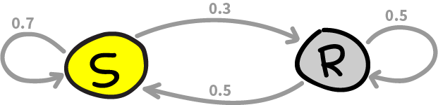
For example, if today is sunny, there is 70% chance that tomorrow is sunny. Otherwise, if today is rainy, there is 50% chance that tomorrow is rainy. Then the transition matrix is given as follows:
$$ Q = \begin{pmatrix} 0.7 & 0.3 \\ 0.5 & 0.5 \end{pmatrix} $$
Note that each row in a transition matrix always sums to 1.
This Markov chain can be visualized as this graph:
n-step transition probability
n-step transition probability is the probability of reaching a state from another state after exactly $n$ steps. We denote it by: $q_{ij}^{(n)} = P(X_{n}=j | X_0=i)$.
Now, consider the 2-step transition probability of a Markov chain. By marginal distribution, we have:
$$ \begin{aligned} q_{ij}^{(2)} &= P(X_{2} = j | X_0 = i) \\ &= \sum_{k=1}^M P(X_{2} = j | X_{1} = k, X_0 = i) P(X_{1} = k | X_0 = i) \\ &= \sum_{k=1}^M q_{kj} q_{ik} = \txt{the} (i, j) \txt{entry of} Q^2 \end{aligned} $$
Similarly reasoning shows that $q_{ij}^{(n)}$ is the $(i, j)$ entry of $Q^n$.
With the weather example above, the matrix representing the 2-step transition probability is given by
$$ Q^2 = \begin{pmatrix} 0.64 & 0.36 \\ 0.6 & 0.4 \end{pmatrix} $$
which implies given that today is sunny, there is 36% chance it will rain two days later.
Note that, in this example, we assume that the transition probability does not change along with time. Such Markov chain is called homogeneous or time-homogeneous.
Marginal distribution of $X_n$
One may ask “What is the probability the system arrives at a specific state at certain time?”. Or what is $P(X_n = j)$?
To calculate this marginal distribution, we need to know the initial conditions of the system. Let $\mathbf{t} = (t_1, …, t_M)$ be the probability vector where $t_i = P(X_0 = i)$, denoting the probability that the system starts at state $i$. Then,
$$ \begin{aligned} P(X_{n} = j) &= \sum_{i=1}^M P(X_0 = i) P(X_{n} = j | X_{0} = i) \\ &= \sum_{i=1}^M t_i q_{ij}^{(n)} = \txt{the }i^{th} \txt{entry of} \mathbf{t}Q^n \end{aligned} $$
So, the marginal distribution of $X_n$ is encoded by $\mathbf{t}Q^n$.
…
Now, you may wonder what $P(X_n = j)$ looks like in the long run. Does it have any special behavior? We will look at it in the next part of the series.